Introduction
The Dream
If you had asked Walt Disney back in 1923 if he thought Cinderella’s castle would be one of the greatest landmarks of childhood imagination, he’d probably say “Who is Cinderella?”. In fact, he didn’t even know if his dream of producing cartoons would come to fruition. After filing for bankruptcy in 1923, Walt moved to Los Angeles to get another shot at entertainment, this time through his brother, Roy Disney. Walt’s second venture, Disney Brothers Cartoon Studio, was founded in October of that same year. By 1926, the studio would get its true name forever: Walt Disney Studios.
The legend of Walt Disney Studios, however, was still in the works. Different trials hit the company like various contractural disputes and staff leaving for other studios. Between all these fires, Walt and one of his favorite animators, Ub Iwerks, came up with their first hit: Mickey Mouse. Mickey Mouse wasn’t just a fun character. He was a live character because of how Walt and Ub adopted new techonology. In 1928, the short Steamboat Willie became the first short that utilized a synchronized soundtrack, effects, music, and dialogue.
Other technical advancements in Disney’s approach to animation helped position it as a disruptor in the industry. Things like Technicolor, multiplane cameras, and a host of other tech adoptions set Disney up to release its first feature film, Snow White and the Seven Dwarfs, in 1937. While some were skeptical of it, the film turned out to be a huge hit, providing the studio with the capital necessary to upgrade its facilities and hit the ground running on more potential hits.
Disney would continue to run into trouble (like WWII) but would continue to persevere, releasing classics like Pinocchio among others. All of these and other creative hits would launch Disney into the prime position to bring the world of imagination from the big screen to real life.
The Big Screen needs a Big Park
While Walt was pleased with the success of the big screen, he knew it was only part of the experience. People didn’t just like watching movies… They wanted to be a part of them! To accomplish this, Walt knew just where to start.
Amusement parks during this time were… sub par to say the least. They were known for being dirty and mechanical. No theme, no flow, just rides and food. While the atmosphere certaintly was still fun, Walt knew that the park could be magical.
In 1948, Walt began outlining plans for Mickey Mouse Park. The initial location for the park was chosen to be in front of their Burbank studios. However, Walt felt the park needed to be much bigger. With the help of Stanford, he found a large area of land in Anaheim to construct his park. Going all in on the park through loans, personal funds, and other means, Walt’s dream of the newly named park, Disneyland, came true in 1955.

While Disneyland hasn’t always been perfect, parents and kids alike have loved being able to immerse themselves in the magic of the movies they love. From Star Wars: Galaxy Edge, to Cinderella’s castle, to a host of other themes, Disneyland continues to set the tone on for theme park experiences.
The Magic behind the Magic: Designing the Flow of the Park
It is estimated that approximately 28 million people visit Disneyland per year. This number is not spread evenly across the year (obviously). Holidays, weather, and other factors play a big role in park attendance. While the park is and will always be about immersing people in the magic of Disney fun, it is not fun to be in an disorganized and chaotic mess. For that reason, the need for proper design of park attractions and placement of park experiencs are crucial in maximizing guest experiences
Let’s for a moment take a look at the park map (we’ll focus on the main Disneyland campus for now).
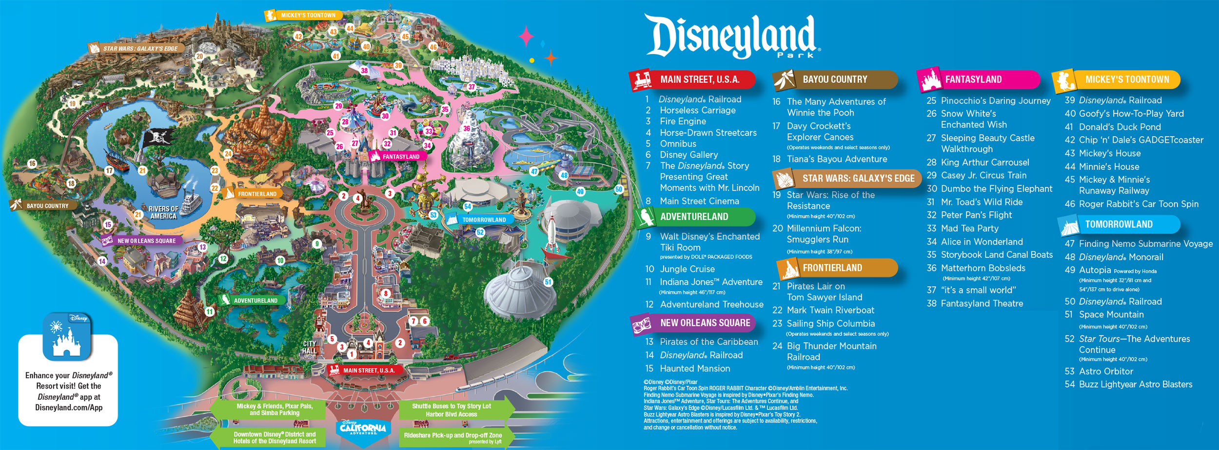
The park is organized in various zones that deal with a common theme. To traverse the park, you need to pass through different zones to get to different attractions (obviously again). Everyone must enter through Main Street and exit from there as well. When attempting to optimize guest experience from this perspective, we need to understand a few important things. To start, how do people usually traverse the park? By understanding “travel” patterns among guests, we can better prepare zones for guest arrivals or properly place entertainment throughout busy routes to “slow traffic”. In short, we want to understand these patterns to have better control on park outcomes. To model this mathematically, we can utilize a graph to visualize this flow.
Using Graphs as a Model
Let G be our graph representation of the park. G then is composed of vertices (or nodes) which we will denote as V and edges which we will denote as E. In this context, G = (V,E). A simple implementation of this framework would be to say that each attraction in the park would be part of our set V and the connecting ways to get to those attractions would be part of our set E. With that in mind, we can utilize this framework to visualize how a crowd moves from specific nodes along certain paths. This is demonstrated in the short video below.
While the number of nodes and people in the park aren’t up to scale, the demonstration of the flow of guests is what we’re after. As already mentioned, everyone begins at the entrance of the park. After that, guests are free to move around the park in whatever process they want. The key insight from this video is that flow doesn’t disappear when people go to an attraction. Flow is just temporarily paused and then released back into the graph. Essentially, once one ride is done, another ride should be expecting inflow.
Returning back to mathematical notation, we call this kind of network a Jackson Network [1]. A Jackson Network essentially is a graph (as shown above) that contains queues. Each node is itself a queue that has its own independent process of arrival and service times. Before getting too deep into the technicals of a Jackson Network, let’s quickly review some basic Queue Theory.
Queue Theory
The nice thing is, everyone has experience a queue so we can all imagine one! Queue theory is simply the mathematical approach to understanding the mechanics behind waiting in line. A queue is generally described in something called Kendall Notation [2], named after the scientist who coined it (obviously). There are three core parts of a queue structure: the arrival process, the service process, and the number of servers. In this post, we’ll assume what most other people assume, which is that the arrival process of park guests follow a poisson process, that service time follows an exponential distribution, and that there is only one server per queue (for ease of math for now).
In Kendall notation, this would be described as a M/M/1 queue (illustrated below).
As shown in the video, the arrival and service process are random according to the probability distribution it follows. In this video, the arrival follows a poisson process with \lambda = 50, which represents 50 customers arriving per hour. The service rate follows an exponential distribution with \mu = 80, meaning the average service rate is 80 customers per hour.
Moving back to the park, the process of the M/M/1 queue is essentially what is happening at each ride in the park (at least in our current simplified view). There is one park operator helping guests onto rides where they arrive in random processes. Once the guests finish their rides, they enter the system again to get into another M/M/1 queue to wait for another ride.
So what’s the point of modeling these lines mathematically? The value is really actually two fold. Using queue theory, we can understand what is currently happening in our system and what we need to improve in the system. For example, let’s take the M/M/1 queue from the video. If in steady state our queue has on average 50 arrivals per hour and can serve on average 80 customers per hour, we can calculate a utilization rate (\rho). This is just the ratio between arrival rate and service rate, which would be 50 over 80, which yields \rho = .625.
Any \rho less than 1 indicates a stable system, meaning the service rate is greater than the arrival rate (i.e. the queue will eventually disappear… phew!). So, from the perspective of park operations, we want to make sure that our queues are stable for each ride. If they aren’t, then we run the risk of super long lines which ruins customer experiences which means bad business.
Graphs with Queues
So far we’ve established that we can model the park as a graph with nodes and edges representing park attractions and pathways between those attractions. We’ve shown that there are mathematial tools that help us quantify the process of arriving, waiting, and being processed at those attractions. We have a model and we have the math that defines the activity within the model. We can now use these together to begin to understand what is happening in the park.
Let’s suppose that we gathered the data in the tables below.
| Ride name | Arrival rate | Service rate |
|---|---|---|
| A | 112 | 121 |
| B | 97 | 121 |
| C | 116 | 135 |
| D | 100 | 102 |
| E | 94 | 96 |
| F | 94 | 119 |
| G | 100 | 110 |
| H | 119 | 136 |
| I | 88 | 112 |
| J | 102 | 102 |
Using the framework of a Jackson Network, we assume that each these queues act independently within the network such that the arrival rates of each ride is the sum of the exit rates of other rides multiplied by the probability of a guest choosing that ride. Mathematically, the arrival rate looks like Equation 2.1.
\lambda_i = \gamma_i + \sum_{j=1}^{J} \lambda_j r_{ji} \quad \text{for } i = 1, 2, \dots, J \tag{2.1}
For example, the arrival rate of ride A is the external arrivals \gamma_i and the expectation (mean) of exit rates from other nodes to ride A. If this is still a bit fuzzy, perhaps a visualization would help. The video below demonstrates a brief simulation using the data from the table.
While a bit chaotic (as an amusement park is as well), the video captures what the data shows. There are certain attractions that have lines that grow much faster than they shrink! For example, ride D’s queue grows from 0 to over 60 by the end of the video. This makes sense because the of the utilization rate of D. D’s utilization rate is a whopping 98%! While the queue won’t grow to infinity, it certainly grows and if it grows, the wait time grows exponentially. We can mathematically view this through Little’s Law[3] shown below.
L = \lambda W \tag{2.2}
The simple formula in Equation 2.2 simply says that the length of the queue is equal to the product between the arrival rate and the wait time of the queue. Rearranging this, we can get the wait time to be W = \frac{L}{\lambda}. If we take the length at the end of the video (60) and divide it by our arrival rate (100), we get .6 hours, or in minutes, 36 minutes. The average wait time (assuming 60 is the long run average) at ride D is 36 minutes! While that might sound like a dream at a place like Disney, it’s not my ideal wait time!
While seeing wait times may be a bit discouraging to park guests, it certainly is a great sight for those running it. Not because park administrators and operators want people waiting in long lines. Rather, the beauty is that they can have baseline metrics to improve the experience! If our park behaves like a Jackson Network, then we can utilize these tools not to just understand how the park is currently working, but how we can manipulate the park to improve customer experience.
From Queue Theory to Operations Management
Up to this point, we’ve covered a lot of math theory to explain the tools that are at our disposal in understanding the physics of guest movement within the park. While we’ll still be utilizing much of the theory, we can now move into the part where we can formulate strategy on how to enhance guest experiences throughout the park.
We know from the table above that we are having issues with the wait time at ride D. The two options we have to help is to either speed up service or slow down flow. Let’s assume that we can’t speed up service right now so our only solution is to slow down flow. How can we do that? Well, since we’re Disney, we can add magic! By that I mean, we should utilize our intellectual property by having our magical guests traverse the park to act as sort of “road blocks”.
Essentially, by strategically placing cast members across the park to slow down flow between rides, we can decrease utilization rates at those rides and subsequently decrease wait time for our guests. Let’s suppose that each guest has a 30% chance of stopping for our cast members. If we place cast members on the path to ride D, we should (in theory) slow flow by about 30%. Let’s see in the video below how this cast member spot slows the flow.
Guests who stop change from red to yellow dots. As we can see, small groups now stop around these attractions. By the end of the video, we ended with 44 guests instead of our previous 60. That’s a 27% decrease in flow to ride D! All with just add some cast members that our guests could say hi to! In theory, we’ve slowed ride attendance by adding guest experiences to the park.
If we can slow flows by adding something as simple as having movie characters walk around the park, what about adding things like gift shops? Food venues? Other fun games? This is essentially the operating model of Disney when it comes to their theme parks. While the rides at attractions provide the “destinations” for the guests, the real money makers are the venues along the way. By providing guests with meaningful experiences and fun gifts along the way to their ride, Disney can both decrease line congestion and bring in more revenue. Don’t believe me? According to Disney’s financials, in 2025 alone, Dinsey brought in about $9 billion in revenue from these in-park sites alone. Not bad for buildings that are meant to slow the flow.
Conclusion
In this post, we covered the history and general business of Disney theme parks. We then dove into the mathematical modeling of the park by showing the park could be defined as a queue network, specifically a Jackson network. We proceeded to walk through some formal definitions of queue models along with their usefulness in defining operations strategy. We utilized these tools to quantify wait time and see if there were ways to help “slow the flow” towards more popular ride destinations.
While the model we presented in this post was valid, it was a VERY simple model of the park. First, we didn’t even include all the rides in the park. Second, we assumed the distances between rides were fairly homogenous. Third, we assumed rides were executed as M/M/1 queue. Fourth, we assumed the park guests were essentially objects that had set probabilities on where to go within the park. In reality, we’d need to step up the model to properly understand the park dynamics. Nonetheless, the point of this point of this point and its simplified model was to introduce readers to the idea of using queue theory to model systems. In that, we can call this post a success.