Abstract
In this post, we present an implementation for Next-Generation Optimization for Dasher Dispatch at DoorDash [1] and Using ML and Optimization to Solve DoorDash’s Dispatch Problem [2]. We demonstrate this implementation in the context of a smaller, simpler food delivery system. We conclude by presenting some simple sensitivity analysis from changes in our hyperparameters weights in our scoring methods. The code for this simulation can be found at the github repo.
Introduction
Food-Ez is a new food delivery service specializing in delivering food in small, walkable cities. Like other companies like DoorDash and UberEats, Food-Ez is a three sided marketplace, dealing with the needs and wants of customers (those who place the orders), restaurants (those who create the orders), and deliverers (those who fulfill the orders). Understanding this, Food-Ez developed a novel dispatch algorithm to maximize efficiency in their marketplace. Specifically, they created an algorithm that minimized delivery time by matching orders to drivers closest to the restaurant. While this approach has been effective for Food-Ez, they are looking to upgrade their current algorithm in a few ways. First, they are allowing deliverers to be assigned up to 2 orders at a time. Second, they want to have more efficient operations. Their current algorithm has drivers waiting quite a bit of time for food to be prepped at restaurants. They want to maximize deliverer efficiency by minimizing driver wait and idle time.
Designing the Problem via Control
Before going into the details of how each algorithm operates within this problem, we first present how to formulate the problem to achieve optimal solutions. One way to approach this problem is by viewing it as a control problem. Control theory offers a rich framework by which we can design our problem and solutions. In essence, control theory aims to stabilize/optimize some system that we’ll denote as P (commonly known as the Plant). The system creates outputs that include feedback signals that are fed back to a controller denoted as C. Figure 3.1 is an example control diagram.
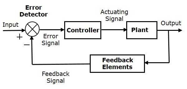
Control theory excels at helping us model dynamical systems and how we can control them even in the face of uncertainty (i.e. not knowing all the dynamics of the system). In our scenario specifically, the delivery marketplace is a highly dynamic system. Orders come in at varying times and locations with an unknown supply of drivers to deliver orders. With control theory, we can boil down this complex problem into essentially three parts: First, what is the system we are trying to control? Second, what information can we gain from the system? Third, what actions can we take to ensure the system operates accordingly?
What’s the system?
The first question can be answered by understanding the business objective. We want customers to utilize our service for their food delivery needs. We promote our service by promising fast and accurate delivery right to their doors. Additionally, since our drivers are critical to the operations of this business, we want to keep our drivers as busy as possible to ensure they maximize earnings. Essentially, our business objective is to maintain optimal customer service to those who order while also providing good opportunities to our deliverers to make money. How can we optimize for both objectives simultaneously? Or rather, what system are we trying to control to fulfill this objective? The system we are aiming to control for Food-Ez is the queue. If we can control the queue (i.e. drive the queue to zero), customers orders will be assigned quickly and be delivered quickly. Subsequently, if the queue is managed correctly, drivers’ objective of maximizing earnings will also be optimized. The queue is the system for which we will be designing a controller.
What should we feedback?
Now that we have identified what the system is, we can identify what elements of the system we should report back to the controller. If we are aiming to optimize the queue, we should report back metrics of queue health. Things like queue length, status of orders, status of drivers, location of dropoff and pickup, etc. The list below enumerates some of the crucial feedback elements we will provide to the controller.
- Order Status (Pending, Assigned, En Route, Delivered)
- Driver Status (Idle, Assigned, En Route, Delivered)
- Order Location (Pickup Location, Dropoff Location)
- Driver Location
- Driver Assigned Orders
For question two, we are essentially defining the states of important elements in our system. In control theory, this fundamental approach is known as representing a system using state-space equations. The formal equations are found in Equation 3.1.
\dot{\mathbf{x}}(t) = \mathbf{A}\mathbf{x}(t) + \mathbf{B}\mathbf{u}(t) \mathbf{y}(t) = \mathbf{C}\mathbf{x}(t) + \mathbf{D}\mathbf{u}(t) \tag{3.1}
Equation 3.1 states that the rate of change of the state vector \dot{x}(t) at time t is equal to the current state vector x(t) multiplied by the dynamics matrix A, plus the input vector u(t) multiplied by the input matrix B. The system’s output, y(t), is equal to the current state vector of the system x(t) multiplied by the output matrix C plus input vector u(t) multiplied by the feedthrough matrix D. Relating these equations back to our control diagram, the controller observes y(t) and compares it against a predetermined reference or baseline. Based on that judgement, the controller sends inputs u(t) back to the system. This input, along with the current state of the system, determines the instantaneous rate of change of the system’s state. This state then produces output y(t), and the process repeats itself.
A classic example of this is cruise control in a car. The controller observes the car’s speed and compares it against the set cruise speed. It then sends inputs to the engine to adjust the speed accordingly. These inputs, alongside other dynamics (e.g., drag, incline), influence the car’s state, which in turn contributes to the measured output y(t).
While these explanations have been incredibly simplified, they illustrate the important principle that a system can be adjusted in a closed-loop by providing crucial feedback to the controller on its current operation. In our scenario, we want to know the locations and destinations of drivers, the status of food preparation, and other relevant parameters, in order to optimally assign orders within the queue and achieve our business objectives.
What actions can we take to adjust the system?
We identified the system and listed some information that would be useful for us to understand how the system is operating. We now need to implement actions that optimize the system’s efficiency. In the previous section(s), we have identified the key objective. We need to assign orders to drivers such that orders get to their locations ASAP while also providing enough work to the drivers. There are several approaches to address this problem and each has its own advantages and disadvantages. We could implement logic such that we always assign the closest driver the order that comes in. Another approach would be holding orders for longer in the queue to see if a more “optimally” positioned driver comes along to take multiple orders nearby. We need sound strategy to identify which algorithmic process we should implement. For Food-Ez, it is optimizing the queue such that we minimize delivery time and maximize driver utilization (i.e. minimize driver idle time). Therefore, we need to design a controller that will balance these two objectives.
Establishing Operations
Before getting into the controller logic, we’ll first walk through the operational flow of our system. This is illustrated in Figure 4.1 (which is provided by [1]).

Walking through Figure 4.1, the process begins with a customer placing an order. The order is processed by the food delivery service and enters the queue. Returning to our control design, the queue sends pertinent information to the controller. The controller “analyzes” the information and sends its “suggested action” back to the queue. The queue then performs the actions by notifying orders to the restaurant (merchant) and sending orders to the “optimal” deliverer (dasher). The order is then picked up by the deliverer and drops off the order.
Once again, we realize the importance of the “controller” in this system. The entirety of the delivery process is determined by the controller. In the next sections, we’ll walk through the previous controller logic and the new proposed controller logic.
Current approach: bipartite matching
The original logic followed by Food-Ez (and additionally DoorDash) was designed by framing the task as a bipartite matching problem. Essentially, this problem involves finding a set of edges in a bipartite graph such that no two edges share a common vertex, thereby matching elements from two distinct sets. In the context of food delivery, this essentially means every order can only have one driver and every driver can only have one order. To do this efficiently to fulfill business objectives such as minimizing delivery time, problems like this can be solved using algorithms like the Hungarian algorithm [3].
While this approach fulfills the business objective, simple examples illustrate the weaknesses of this approach. Suppose a deliverer is assigned an order and is heading to the restaurant. On the way, the driver passes another restaurant that just received an order that will be ready shortly. Furthermore, the dropoff location of this order is nearby the dropoff location of the first order. Instead of assigning this order to the driver, the system must assign another driver to this order. While more drivers are utilized in this approach, drivers could be used more efficiently.
An example via queue theory
To illustrate this, let’s pose the simple scenario of a single deliverer working for Food-Ez. Utilizing queue theory, we’ll assume this is an M/M/1 queue where the arrival process is modeled by a Poisson distribution with parameter \lambda = 1 (per hour), the service distribution is an exponential distribution with \mu = 2 (per hour), and there is a single server (deliverer).
With these metrics, we can calculate system utilization (or driver utilization in our case). This is defined as \rho = \frac{\lambda}{\mu}, or the ratio between arrival rate and service rate. In our case, for a deliverer in the bipartite matching system, we get 50% driver utilization. While this is not bad, the average queue wait time for an order is defined as W_{q} = \frac{L_{q}}{\lambda}, where L_{q} is average length of queue. The average length of the queue here is .5 so in our scenario, queue wait time is about .5 hours or 30 minutes. Since our deliverer can only handle one order at a time, every order on average would have to wait 30 minutes in the queue.
In a different approach, let’s say a deliverer can now take two orders concurrently and assume it is no further than a 10 minute drive to complete. In this case, a deliverer can fulfill 2 orders in about 40 minutes (1 order / 30 mins was the rate before). Converting this to hours, a deliverer can now fulfill 3 orders per hour, thus changing our deliverer utilization rate from 50% to 33%. More importantly, the queue wait time decreases from 30 minutes to 10 minutes (average queue length in this scenario is ~.167 orders, which is then divided by 1 order per hour). Not only could our drivers stay more busy if arrival rates increased, but our customers would have to wait only a third of the old time (if our simple assumptions hold)!
Optimizing Dispatch using Integer Programming
So far we have demonstrated from a high-level the current operations of Food-Ez: a customer places an order, the controller (using a dispatch algorithm) matches orders to restaurants and deliverers to orders such that we minimize delivery time from order placement to order delivery. To accommodate other business objectives, we need a new optimization framework for our dispatch algorithm. Once implemented, we can substitute the current dispatch algorithm for the newly enhanced one and it should fit into our control design seamlessly. Our proposed solution for accomodating multiple business objectives is integer programming with a weighted sum score [4] (Note: [1] uses a mixed integer program approach due to the more complex and wholistic approach to addressing the dispatch problem, but for our simple scenario, we reduce the problem to an integer program). Our formulation is found in Equation 5.1.
\min_{x} \sum_{i=1}^{N}\sum_{j=1}^{D} c_{ij(t)}x_{ij} \sum_{j=1}^{D} x_{ij} = 1 \; \forall i \in \{1, \dots, N\} \sum_{i=1}^{N} x_{ij} \le 2 \; \forall j \in \{1, \dots, D\} \tag{5.1}
c_{ij}(t) = \sum_{m=1}^{W} w_{m}p_{m} \tag{5.2}
Let N be the set of unassigned orders and let D be the set of available drivers. We filter these sets such that only orders not yet assigned (orders can only be assigned and accepted once) and drivers with fewer than two active orders are considered. Once we have our viable sets, we aim to minimize the cost function (objective function) where c_{ij} is the cost associated with assigning the ith order to the jth driver. x_{ij} is the decision variable in our program, which is a binary variable of whether we assign the ith order to the jth driver. The cost associated with each order is determine by Equation 5.2, where we define the cost as a weighted sum of different predictors. In our scenario with Food-Ez, we define four key variables below.
- Route Time (total time duration of driver arriving to restaurant, picking up the order, and dropping off the order)
- Wait Time (total prep time of the order)
- Drive Acceptance (probability of a driving accepting an order)
- Driver Idleness (binary of whether or not driver has any orders or no)
This new approach allows us to determine which of our four factors are most pressing for our current business needs since we can adjust the weights of these accordingly and allow the objective function to recognize those changes. For the complete code up of our algorithm, see the github repo.
Simulation Results
We have successfully defined a new approach for our Food-Ez dispatch algorithm. To assess its efficacy in real-world scenarios, we designed a simulation to test it. We ran 5 simulations for 120 iterations (120 simulation “minutes”). The simulation parameters consist of the following: number of drivers (which we hold constant throughout), number of restaurants, grid size of city, order arrival rate, route time weight, wait time weight, driver acceptance weight, and driver idleness weight. Each simulation with their respective parameters are found below.
- Simulation(10, 10, 5, 1, .5, .2, .1, .2)
- Simulation(5, 10, 5, 1, .5, .2, .1, .2)
- Simulation(10, 10, 5, 1, .05, .7, .05, .2)
- Simulation(10, 10, 5, 1, .25, .25, .25, .25)
- Simulation(10, 10, 5, 1, .8, .05, .1, .05)
For example, simulation 1 has 10 drivers with 10 restaurants, a city that is 5x5 units, an order arrival rate of 1 (per minute), .5 weight on route time, .2 weight on wait time, .1 weight on driver acceptance, and .2 weight on driver idleness. The results of each simulation is found below in Table 6.1. (Note: we ran each simulation with the same random seed settings for consistency in comparison).
| Simulation | Orders | Pending | Assigned | En Route | Delivered | Avg Driver Wait Time | Avg Driver Idle Time | Avg Time To Pickup | Avg Time To Dropoff | Avg Time Of Total Route | Avg Time Pending |
|---|---|---|---|---|---|---|---|---|---|---|---|
| 1 | 120 | 0 | 7 | 1 | 112 | 21.50 | 59.50 | 6.78 | 1.73 | 8.52 | 0.40 |
| 2 | 120 | 0 | 6 | 1 | 113 | 71.40 | 2.80 | 6.00 | 1.00 | 7.00 | 0.00 |
| 3 | 120 | 0 | 7 | 1 | 112 | 53.20 | 41.30 | 6.24 | 1.13 | 7.38 | 0.42 |
| 4 | 120 | 0 | 7 | 1 | 112 | 31.90 | 51.00 | 6.32 | 1.64 | 7.96 | 0.25 |
| 5 | 120 | 1 | 6 | 2 | 111 | 19.40 | 61.00 | 6.73 | 1.76 | 8.50 | 0.32 |
From Table 6.1, the number of deliveries performed appear to be consistent even with the change of parameter weights. This is a nice observation since simulation 2 had half of the drivers that the other simulations had, but delivered the most orders. Furthermore, simulation 2 shows that drivers were used efficiently as most drivers were only idle for on about 3 minutes on average, compared to the other simulations that had far more idle time. We continue to see this trend in other metrics for simulation 2. Simulation 2 had the lowest average time to dropoff, lowest average time of total route, and even lowest pending time for orders in the queue. Further investigation is needed to see what the optimal driver supply would be in different scenarios, but this is a telling sign at the moment that our new algorithm utilizes driver supply more efficiently.
There are many other interesting findings from these 5 simulations, but we will leave these to the reader to discover.
Conclusion
In this post, we presented a business case where a food-delivery company, Food-Ez, is looking to optimize their dispatch algorithm to accomodate more business objectives. We then walked through how this problem can be designed as a control problem and identified the system to be controlled, the feedback data needed to control it, and how to design our controller.
Our controller in this scenario is the dispatch algorithm itself, designed to more efficiently assign orders by raising the limit on orders a driver can carry along with other business objectives within our objective function. To do this, we changed our algorithm foundation from a bipartite matching problem to an integer programming program. We formulated how we would minimize this new objective function and designed a simulation to demonstrate the usefulness of it.
Next steps would include further simulations with more “real-world” dynamics involved and potential experimentation using things like switchback experiments. Overall, we hope this post demonstrated key frameworks that one can use in designing real-world applications to enhance operational efficiency for businesses.