1 What are your beliefs?
In his book Leading with the Heart, Coach Krzyzewski lays out in the early chapters the importance of establishing an identity for any team. He credits a lot of this thought to his familiar upbringing where his parents instilled in him and his siblings the importance of family values. He also credits a lot of this to his military training where each member of a unit knew the importance of knowing their role to play in the success of an assignment. In short, who Coach Kryzyewski was drove a lot of how he ran his basketball team. Integrity was an important principle on the team because he valued it in his own life, and the list goes on of how he built his teams around these common attributes.
Coach Kryzewski isn’t the only one who does this. Everyone has beliefs that influence how they approach work. The trick though is identifying what those beliefs are in order to check if the actions we are performing are aligned with the values we espouse having.
In 1954, statistician Leonard J. Savage published The Foundations of Statistics [Savage1954]. In this work, Savage introduced several models demonstrating how subjective beliefs influence decision-making. The most notable of these models is Subjective Expected Utility (SEU), shown in Equation 1.1.
\[ U(f) = \int_{S} u(f(s)) p(s) \, ds \tag{1.1}\]
Breaking down the formula a bit, we say that the expected utility of an individual (\(U(f)\)) is equal to the integral of the state space \(S\), the utility function \(u(f(s))\), and the subjective probability density function (PDF) \(p(s)\). What this “complex” formula is essentially saying is that we make decisions based on our perceived values and our current information. The perceived values are represented via the utility function as that mathematically maps our tastes and preferences to a more “measurable” area. The PDF is how we currently perceive how likely our outcomes are that derive our utility.
That was a lot of mathematic and economic jargon, so let’s move into an example that most people can relate to: what is the quickest way to get home. Let’s pose for a moment that we don’t have google maps to tell us which route is the “quickest” way to get home. As well, let’s suppose there are only two ways to get home: via the freeway or through town. Your utility is highest when your commute is as short as possible (ie by minimizing your commute time, you maximize utility). You know that the freeway is the fastest way to get home, but you believe there is about a 30% chance that there is an accident on the freeway and that would slow things down considerably. The other way through town is the slowest option, but you know that there is only about a 5% chance there is an accident. Which way would you choose?
This is the SEU model in action. We all have “imperfect” information (\(p(s)\)) along with personal preferences (\(u(f(s))\)) that drive our decisions. Recognizing this and formalizing it in a mathematical model helps us to do two things: understand what our current beliefs are and what we currently decide based on those decisions.
Our beliefs, as shown in the SEU, are represented as probability distributions. This merely means that we can take on a range of values that express how certain, or uncertain, we are about a given event.
In the context of basketball, this is demonstrated in a plethora of ways that we’ll get into later on in the book, but the important principle to understand is that beliefs drive the creation and pursuit of systems.
1.1 Updating Beliefs: The Power of Bayesian Thinking
An important example of this is the development of a gameplan. Coaches watch lots of film to understand the tendencies, strengths, and weaknesses of each team they compete against. Before watching the film, your beliefs about a given team can be fairly broad. You may have heard the team shoots a lot of three or likes feeding the post, etc. Once you engage with material that potentially reinforces this idea, your uncertainty decreases and you are more “willing” to commit to certain actions since you know they more than likely would happen. If you were unsure that someone on the opposing team would still shoot even on a closeout but watching film you see repeatedly they are a quick trigger, you are more certain that this would be a viable strategy to defend against them.
This doesn’t only happen in pre-game planning. This happens during the game as you adjust your players, offense, and defense matchups according to new information you perceive over the course of the game.
Mathematically, this can be modeled using Bayesian statistics. The story on how Bayesian statistics came to be essentially goes like this. Back in the 1700s, an english minister by the name of Thomas Bayes wanted to essentially prove that the resurrection occurred. To do this, he asked a profound question: if you don’t know the certainty of an event, how can you calculate the probability of that event happening given observed events? This led Bayes to publish his paper An Essay towards solving a Problem in the Doctrine of Chances [1] where he formalized this phenemon. That is, as people see new evidence on a particular matter, their beliefs are updated based on the strength of the evidence.
In the game of basketball, this is crucial to recognize, especially as a coach. Let’s walk through the mathematics of this using some visualizations. Let’s say that you are preparing to play a team that is great at moving the ball. They’re an unselfish team that excels at making sure everyone touches the ball before a shot attempt. You want to understand how often they pass because you think that if you can accurately “predict” on what number pass they will attempt to shoot, you can better prepare your defense for a shot and subsequent rebound attempt.
A simple way we could model this is using a Poisson distribution. Poisson distributions are handy for calculating the number of discrete events that take place in a given period of time (in our case, a single half-court possession). The probability mass function (PMF) for the Poisson distribution is shown below.
\[ P(k \mid \lambda) = \frac{\lambda^k e^{-\lambda}}{k!} \tag{1.2}\]
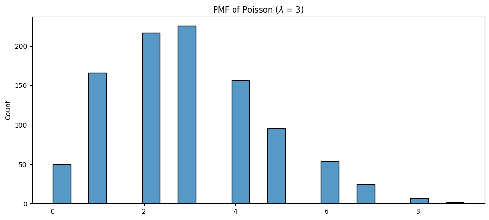
This PMF simply states that the probability that we observe \(k\) number of passes given a distribution parameter \(\lambda\) is equal to what you see in Equation 1.2. For example, below is the PMF where \(\lambda\) = 3.
The plot above merely shows the frequency each value \(k\) should occur based on our belief that the average frequency (\(\lambda\)) is equal to 3. The most frequent value here is 3 which makes sense since that is the average of this kind of distribution. To get a probability from this, just plug the value \(k\) into the equation Equation 1.2. Using that, we get the probability of the team making exactly 3 passes in a given possession to be ~22%.
But how certain are you that the average number of passes is exactly 3? How much data have you collected that would show that they always have this kind of distribution for number of passes in a given offesnive possession? This is where Bayesian updating comes in. We don’t have to stick with just 3 \(\lambda\) parameter. We can have lambda take on a whole distribution of values that represent our uncertainty about it. The way we model this is shown in Equation 1.3.
\[ P(\lambda | D) = \frac{P(D | \lambda) P(\lambda)}{P(D)} \tag{1.3}\]
The equation above is what we discussed earlier with Sir Thomas Bayes. In words, Equation 1.3 states that our beliefs are updated based on new data we receive. In the context of our basketball scouting, our belief of the average number of passes in a given offensive possesion \(\lambda\) is updated by the data we receive \(D\) through a simple ratio. The numerator is the product between our prior beliefs \(P(\lambda)\) and the likelihood of our beliefs \(P(D|\lambda)\) divided by the probability of observing the data \(P(D)\).